Excel

SOME EXCEL STUFF

Our process starts by giving the client the ability to create any peer group(s) of investments around any mutual funds, ETFs, closed-end, private portfolios and custom portfolios.

We create custom benchmarks according to our client’s (and their investors) world-view.

We maintain a terabyte-size proprietary 1940-act fund operations and performance database to research a wide array of subjects, from r-square performance attribution to effective advisory fees.

Past research includes:

• Administration fee comparisons
• Advisory metrics
• Performance fee models
• Legal costs
• Sales and redemption analysis
• Portfolio Commissions
• Start-up funds
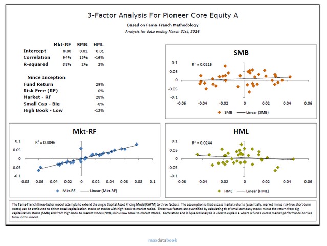
• 3-factor tracking
• New funds data

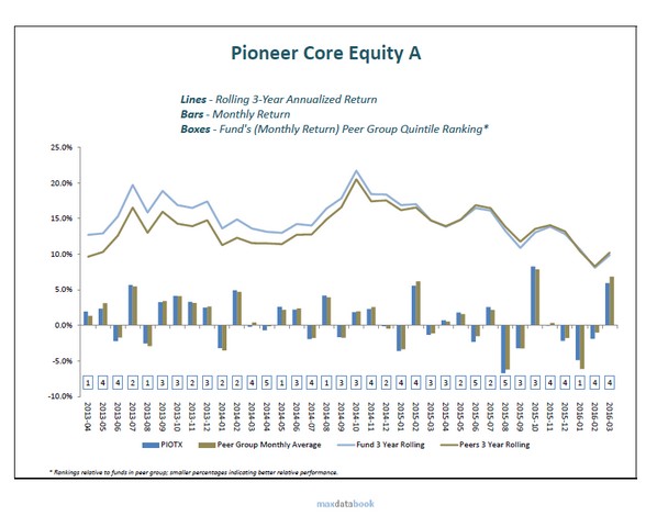
Here’s some sample VBA I wrote to enhance an Excel chart.  The following chart is not built-in to Excel; that is, I had to develop, or program, a custom routine to add the quartile / quintile boxes on the right.

VBA code…

Sub ab00_CHART_RelativePerfRanking_ALL_RUN_nTile()

Dim iDataRowStart As Integer
Dim iDataRowEnd As Integer
Dim sDataSeries As String
Dim dFunds As New Dictionary
Dim xFunds As Variant
Dim sChartCaption As String

Dim sDataSheet As String

' ***** CONFIG ********************
sDataSheet = "DATA_PerformanceRankings"
' Fill working fund dictionary list
Dictionary_Fill_gdRA_MasterListColVals 2 ' 1 would be ticker
' Quartile (4) or Quintile (5), or other?
nTile = 5
' *********************************

' ***
' Create 1-Year Charts (cols E,F,G)
' ***
   For Each vKey In gdRA_MasterListColVals.Keys
    ' GET FUND ... RA_MasterList data
  
    vxcols = Split(gdRA_MasterListColVals.Item(vKey), "|")
    sFund = vxcols(1) ' would be short name we use for sheet name
    PeerGroup = vxcols(0) ' 1st col, PeerGroup
    ' Find where the fund's data block begins (row number)
    iDataRowStart = SheetRowGetNum(sDataSheet, "A1", PeerGroup)
     
    If iDataRowStart > 0 Then
    
    vCheckHasData = Sheets("DATA_PerformanceRankings").Range("E" & iDataRowStart).Value + _
        Sheets("DATA_PerformanceRankings").Range("F" & iDataRowStart).Value + _
        Sheets("DATA_PerformanceRankings").Range("G" & iDataRowStart).Value + _
        Sheets("DATA_PerformanceRankings").Range("H" & iDataRowStart).Value
    
        If vCheckHasData > 0 Then
        
        sDescription = Sheets("DATA_PerformanceRankings").Range("D" & iDataRowStart).Value
        If InStr(sDescription, "Lipper") > 0 Then
        sChartCaption = "* Rankings relative to selected peer group; smaller percentages indicating better relative performance"
            Else
            sChartCaption = "* Rankings relative to selected peer group; smaller percentages indicating better relative performance"
        End If
            
        ' Now create chart Sheet, RangeStart, ChartName, Left, Top, sDataSeries
        ' POSITION: TOP/LEFT
        ' 5.25, 123, (4.6 * 72), (2.75 * 72),
        ab00_CHART_RelativePerfRankings_Draw_nTile sDataSheet, _
            "A", _
            iDataRowStart, _
            sFund, "I7", "RelPerfRank", 339, 80.25, _
            sDataSeries, "2015 Relative Performance Ranking* (% and quintile)", _
            sChartCaption, nTile
        
            Else
            
            currSheet = ActiveSheet.Name ' get current sheet name to go back to
            ' go to chart sheet
            Sheets(sFund).Select
            CHARTS_DrawBox_PerfRankingsMissing
            Sheets(currSheet).Select ' now back to where we were
            
        End If
    
    End If 'exist
    
    Next

Range("a3").Select

End Sub

Sub ab00_CHART_RelativePerfRankings_Draw_nTile(argDataSheet, argDataCol, argDataRow, _
    argSheet, argCellPositionFirst, argChartName, argL, argT, sSeriesData, argTitle, argChartCaption, argnTile)

' ****** GET CHART DATA **************
Dim sR1 As String
' Add bank for reference
Dim sDataSheet As String
sDataSheet = "=" & argDataSheet & "!"
' We'll need 3 rows, so make strings for them
sR1 = Trim(Str(argDataRow)) ' First Row, was +3 for original type

' And we'll need 3 series (name/value pairs)
Dim s1N, s1V, sXlegend As String
' Legend same for all
sXlegend = sDataSheet & "$E$1:$G$1"

' Legend same for all
sXlegend = sDataSheet & "$E$1:$G$1"

'"Data_1_3_5_10_Year").Range("E5:H5"
s1N = sDataSheet & "$E" & sR1 & ":G" & sR1
s1V = sDataSheet & "$E$" & "1" & ":$G$" & "1"  ' prob won't use this

' Let's pass these pack as one pipe-deliminated string
sSeriesData = s1N & "|" & s1V & "|" & sXlegend

' ******* END GET CHART DATA *************

Sheets(argSheet).Select
Range(argCellPositionFirst).Select

' DELETE

NumCharts = ActiveSheet.ChartObjects.Count
    For ic = NumCharts To 1 Step -1
        If ActiveSheet.ChartObjects(ic).Name = argChartName Then
        ActiveSheet.ChartObjects(ic).Delete
        End If
    Next ic

'
Dim xSeriesData
xSeriesData = Split(sSeriesData, "|")

' Now go to range where we want to create chart (though we'll really use Left/Top coordinates)
Range(argCellPositionFirst).Select

    ActiveSheet.Shapes.AddChart.Select
    ActiveChart.Parent.Name = argChartName ' Name Chart
    ActiveChart.ChartType = xlColumnClustered
    ActiveChart.ClearToMatchStyle
    ActiveChart.ChartStyle = 3
    ActiveChart.ClearToMatchStyle
    ' Get Data
    ActiveChart.SeriesCollection.NewSeries
    ActiveChart.SeriesCollection(1).Name = xSeriesData(1) '"=Data_1_3_5_10_Year!$D$2" ' Series 1 Name
    ActiveChart.SeriesCollection(1).Values = xSeriesData(0) '"=Data_1_3_5_10_Year!$F$2:$F$2" ' Series 1 Values
    
    'ActiveChart.SetSourceData Source:=Sheets("Data_1_3_5_10_Year.Range("E5:H5")") '"(Data_1_3_5_10_Year").Range("E5:H5)"
    ActiveChart.SeriesCollection(1).xValues = xSeriesData(2) '"=Data_1_3_5_10_Year!$E$1:$H$1"
    
    ' Change Scale 1 to 0 in .25s
    ActiveChart.Axes(xlValue).Select
    ActiveChart.Axes(xlValue).MinimumScale = 0
    ActiveChart.Axes(xlValue).MaximumScale = 1
    ' Either Quartile or Quintile For now
    If argnTile = 4 Then
    ActiveChart.Axes(xlValue).MajorUnit = 0.25 ' QUARTILES
        Else
        ActiveChart.Axes(xlValue).MajorUnit = 0.2 ' QUINTILES
    End If
    ActiveChart.Axes(xlValue).TickLabels.NumberFormat = "0%"
        
    ' Reverse, from top down
    ActiveChart.Axes(xlValue).ReversePlotOrder = True
    Selection.MajorTickMark = xlNone
    
    ' Change Column Widths
    ActiveChart.SeriesCollection(1).Select
    ActiveChart.ChartGroups(1).Overlap = 100
    ActiveChart.ChartGroups(1).GapWidth = 35
    
    ' Change colors
    With Selection.Format.Fill
       ' RBB Method works
       ' .Visible = msoTrue
       ' .ForeColor.RGB = RGB(0, 128, 128)
       ' .Transparency = 0.4392156601
       ' .Solid
       .ForeColor.ObjectThemeColor = msoThemeColorAccent5
       .ForeColor.TintAndShade = 0
       .ForeColor.Brightness = -0.25
       .Transparency = 0.4392200112
    End With
    
    ' Add Chart Titles
    ' Can't RESIZE CHART TIEL WIDTH SO DO BOX INSTEAD
    ActiveChart.SetElement (msoElementChartTitleCenteredOverlay)
    Selection.Caption = "" 'argTitle ' like "One Year Performance"
    'ActiveChart.ChartTitle.Select
    'Selection.Format.TextFrame2.TextRange.Font.Size = 12
    
    ' TITLE BOX
ActiveChart.Shapes.AddTextbox(msoTextOrientationHorizontal, _
    17, _
    0.3, _
    315, _
    22).Name = "TBTitle"
    ActiveChart.Shapes("TBTitle").Select
    Selection.Height = 22
    Selection.ShapeRange.TextFrame2.TextRange.Font.Size = 11
    Selection.ShapeRange("TBTitle").TextFrame2.TextRange.Characters.Text = argTitle '"2013 Relative Performance Ranking (% and quartile)*"
    ActiveChart.Shapes.Range(Array("TBTitle")).Select
    Selection.ShapeRange.TextFrame2.TextRange.Font.Bold = msoTrue
    Selection.ShapeRange.TextFrame2.TextRange.ParagraphFormat.Alignment = _
    msoAlignCenter
    
    Selection.ShapeRange.TextFrame2.TextRange.Font.Fill.ForeColor.ObjectThemeColor = msoThemeColorAccent5
    Selection.ShapeRange.TextFrame2.TextRange.Font.Fill.ForeColor.TintAndShade = 0
    Selection.ShapeRange.TextFrame2.TextRange.Font.Fill.ForeColor.Brightness = -0.5
  
   
   'set focus back to chart
    ActiveSheet.ChartObjects(ActiveChart.Parent.Name).Activate
    
    ' Put data lables inside bars
    ActiveChart.SeriesCollection(1).ApplyDataLabels
    ActiveChart.SeriesCollection(1).DataLabels.Select
    Selection.Position = xlLabelPositionInsideEnd
    
    ' Put legends at bottom (years)
    ActiveChart.Axes(xlCategory).Select
    Selection.TickLabelPosition = xlHigh
    
    ' Turn off ticks
    Selection.MajorTickMark = xlNone
    
    ' Delete data legend
    ActiveChart.Legend.Select
    Selection.Delete
    
    ' Delete any data values THAT ARE 0 !
    Dim vxVals As Variant
    vxVals = ActiveChart.SeriesCollection(1).Values
   
    If vxVals(1) = 0 Then
    ActiveChart.SeriesCollection(1).DataLabels.Select
    ActiveChart.SeriesCollection(1).Points(1).DataLabel.Select
    Selection.Delete
    End If
    
    If vxVals(2) = 0 Then
    ActiveChart.SeriesCollection(1).DataLabels.Select
    ActiveChart.SeriesCollection(1).Points(2).DataLabel.Select
    Selection.Delete
    End If
    
    If vxVals(3) = 0 Then
    ActiveChart.SeriesCollection(1).DataLabels.Select
    ActiveChart.SeriesCollection(1).Points(3).DataLabel.Select
    Selection.Delete
    End If
    
      ' We between 5% and 15% let's scootch label down a bit
    If vxVals(3) >= 0.05 And vxVals(3) <= 0.15 Then ActiveChart.SeriesCollection(1).DataLabels.Select ActiveChart.SeriesCollection(1).Points(3).DataLabel.Select Selection.Top = Selection.Top + 17 End If If UBound(vxVals) > 3 Then
    If vxVals(4) = 0 Then
    ActiveChart.SeriesCollection(1).DataLabels.Select
    ActiveChart.SeriesCollection(1).Points(4).DataLabel.Select
    Selection.Delete
    End If
    
    ' We between 5% and 15% let's scootch label down a bit
    If vxVals(4) >= 0.05 And vxVals(4) <= 0.15 Then
    ActiveChart.SeriesCollection(1).DataLabels.Select
    ActiveChart.SeriesCollection(1).Points(4).DataLabel.Select
    Selection.Top = Selection.Top + 17
    End If
    End If '
    
    ' set focus back to chart
    ActiveSheet.ChartObjects(ActiveChart.Parent.Name).Activate
    
    ' Change grid lines to light gray
    ActiveChart.Axes(xlValue).MajorGridlines.Select
    With Selection.Format.Line
        .Visible = msoTrue
        .ForeColor.ObjectThemeColor = msoThemeColorBackground1
        .ForeColor.TintAndShade = 0
        .ForeColor.Brightness = -0.349999994
        .Transparency = 0.5
    End With
    
    ' Resize to fix boxes
    ' CHANGE CHART WIDTH AND HEIGHT
    ' Points, Approx 1/72nd of an Inch
    ActiveChart.Parent.Width = (4.6 * 72) '330
    ActiveChart.Parent.Height = (2.35 * 72) '169
 
    ActiveSheet.ChartObjects(ActiveChart.Parent.Name).Activate
    
    ActiveChart.PlotArea.Height = 132 ' height before top
    ActiveChart.PlotArea.Width = 272
    
    ActiveChart.PlotArea.Left = 4
    ActiveChart.PlotArea.Top = 18
    
    'First positioning
    ActiveChart.Parent.Left = argL
    ActiveChart.Parent.Top = argT
    
    ' *********************************************
    ' COLOR CODED PERCENTILE TEXT BOX DRAWING
    ' *********************************************
    
    ' We need to get values to start adjusting
    Dim vChartName
    Dim vChartHeight
    Dim vChartWidth
    Dim vChartLeft
    Dim vChartTop
    Dim vChartPlotHeight
    Dim vChartPlotWidth
    Dim vChartPlotLeft
    Dim vChartPlotTop
    
    vChartName = ActiveChart.Parent.Name
    vChartWidth = ActiveChart.Parent.Width
    vChartHeight = ActiveChart.Parent.Height
    vChartLeft = ActiveChart.Parent.Left
    vChartTop = ActiveChart.Parent.Top
    vChartPlotWidth = ActiveChart.PlotArea.Width
    vChartPlotHeight = ActiveChart.PlotArea.Height
    vChartPlotLeft = ActiveChart.PlotArea.Left
    vChartPlotTop = ActiveChart.PlotArea.Top
    
    If argnTile = 4 Then
    
    ' Text Box 1
    argName = "TB1"
    argText = "1st"
    argLeft = 5 + vChartPlotWidth + 1
    argTop = ActiveChart.PlotArea.Top + 6
    argWidth = (ActiveChart.PlotArea.Height / 4) - 7 ' 6 for grid lines?
    argHeight = argWidth + 0.2
    argR = 0
    argG = 176
    argB = 80
    
    ' Now we have height, can change width
    argWidth = argWidth + 5.4
    
    CHART_Create_TextBox argName, argText, argLeft, argTop, argWidth, argHeight, argR, argG, argB, argTextColor
    
    argName = "TB2"
    argText = "2nd"
    argTextColor = "Black"
    argHeight = argHeight + 0.5
    argR = 146
    argG = 208
    argB = 80
    ' Next textbox, top is box on top top + height
    argTop = argTop + argHeight - 0.02
    ' Everything else stays same
        On Error Resume Next
        ActiveChart.Shapes(argName).Delete
        On Error GoTo 0
    CHART_Create_TextBox argName, argText, argLeft, argTop, argWidth, argHeight, argR, argG, argB, argTextColor
    
    argName = "TB3"
    argText = "3rd"
    argHeight = argHeight
    argR = 238
    argG = 232
    argB = 0
    ' Next textbox, top is box on top top + height
    argTop = argTop + argHeight
    ' Everything else stays same
        On Error Resume Next
        ActiveChart.Shapes(argName).Delete
        On Error GoTo 0
    CHART_Create_TextBox argName, argText, argLeft, argTop, argWidth, argHeight, argR, argG, argB, argTextColor
    
    argName = "TB4"
    argText = "4th"
    argHeight = argHeight - 0.2
    argR = 138
    argG = 0
    argB = 0
    argTextColor = "White"
    ' Next textbox, top is box on top top + height
    argTop = argTop + argHeight
    ' Everything else stays same
        On Error Resume Next
        ActiveChart.Shapes(argName).Delete
        On Error GoTo 0
    CHART_Create_TextBox argName, argText, argLeft, argTop, argWidth, argHeight, argR, argG, argB, argTextColor
    
    
        Else
        ' *********
        ' QUINTILES
        ' *********
    
    ' Let place a box to right of plot area
    argName = "TB1"
    argText = "1st"
    argLeft = 5 + vChartPlotWidth + 1
    ' QUARTILE
    'argTop = ActiveChart.PlotArea.Top + 6
    ' QUINTILE
    argTop = ActiveChart.PlotArea.Top + 6
        ' QUARTILE
    'argWidth = (ActiveChart.PlotArea.Height / 4) - 7 ' 6 for grid lines?
    ' QUINTILE
    argWidth = (ActiveChart.PlotArea.Height / 5) - 7 ' 6 for grid lines?
    
    'Debug.Print argWidth
    ' QUART
    'argHeight = argWidth + 0.2
    ' QUINT
    argHeight = argWidth + 0.5
    
    ' Now we have height, can change width
    argWidth = argWidth + 5.4
        
    ' TextBox 1
    argR = 0
    argG = 153
    argB = 0
    CHART_Create_TextBox argName, argText, argLeft, argTop, argWidth, argHeight, argR, argG, argB, argTextColor
    
    ' QUINTILES !!!! QWER
    argName = "TB2"
    argText = "2nd"
    argTextColor = "Black"
    argHeight = argHeight
    argR = 146
    argG = 208
    argB = 80
    ' Next textbox, top is box on top top + height
    argTop = argTop + argHeight + 1.35
    ' Everything else stays same
        On Error Resume Next
        ActiveChart.Shapes(argName).Delete
        On Error GoTo 0
    CHART_Create_TextBox argName, argText, argLeft, argTop, argWidth, argHeight, argR, argG, argB, argTextColor
    
    argName = "TB3"
    argText = "3rd"
    argHeight = argHeight
    argR = 255
    argG = 255
    argB = 153
    ' Next textbox, top is box on top top + height
    argTop = argTop + argHeight + 1.35
    ' Everything else stays same
        On Error Resume Next
        ActiveChart.Shapes(argName).Delete
        On Error GoTo 0
    CHART_Create_TextBox argName, argText, argLeft, argTop, argWidth, argHeight, argR, argG, argB, argTextColor
    
    argName = "TB4"
    argText = "4th"
    argHeight = argHeight
    argR = 255
    argG = 192
    argB = 0
    argTextColor = "Black"
    ' Next textbox, top is box on top top + height
    argTop = argTop + argHeight + 1.35
    ' Everything else stays same
        On Error Resume Next
        ActiveChart.Shapes(argName).Delete
        On Error GoTo 0
    CHART_Create_TextBox argName, argText, argLeft, argTop, argWidth, argHeight, argR, argG, argB, argTextColor
    
    ' QUINT
    argName = "TB5"
    argText = "5th"
    argHeight = argHeight
    argR = 192
    argG = 0
    argB = 0
    argTextColor = "White"
    ' Next textbox, top is box on top top + height
    argTop = argTop + argHeight + 1.35
    ' Everything else stays same
        On Error Resume Next
        ActiveChart.Shapes(argName).Delete
        On Error GoTo 0
    CHART_Create_TextBox argName, argText, argLeft, argTop, argWidth, argHeight, argR, argG, argB, argTextColor
    
    End If 'Quartile or Quintile boxes
    
     ' *****************
    ' ADD FOOTNOTE
    ' *****************
    Dim sFootnote As String '
    sFootnote = argChartCaption '"* Rankings relative to investment category with smaller percentages indicating better relative performance"
    ActiveChart.Shapes.AddTextbox(msoTextOrientationHorizontal, 5, 147, 310, 12).Select
    Selection.ShapeRange.TextFrame2.TextRange.Font.Size = 7
    Selection.ShapeRange.TextFrame2.TextRange.Font.Italic = True
    Selection.ShapeRange(1).TextFrame2.TextRange.Characters.Text = sFootnote
    Selection.ShapeRange(1).TextFrame2.TextRange.Characters(1, Len(sFootnote)).ParagraphFormat. _
        FirstLineIndent = 0
        
    ' Format Chart Box
    ActiveChart.ChartArea.Select
    With ActiveSheet.Shapes("RelPerfRank").Line
        .Visible = msoTrue
        .ForeColor.ObjectThemeColor = msoThemeColorBackground1
        .ForeColor.TintAndShade = 0
        .ForeColor.Brightness = -0.150000006
        .Transparency = 0
    End With
    ActiveChart.ChartArea.Select

        
    Range("A1").Select
        
    
End Sub

Sub CHART_Create_TextBox(argName, argText, argLeft, argTop, argWidth, argHeight, argR, argG, argB, argTextColor)

' Create TEXTBOX L,T,W,H
ActiveChart.Shapes.AddTextbox(msoTextOrientationHorizontal, _
    argLeft, _
    argTop, _
    argWidth, _
    argHeight).Name = argName
ActiveChart.Shapes(argName).Select

' Color fill
    Selection.ShapeRange.TextFrame2.VerticalAnchor = msoAnchorMiddle
    With Selection.ShapeRange.Fill
        .Visible = msoTrue
        .ForeColor.RGB = RGB(argR, argG, argB) ' DARK GREEN
        .Transparency = 0.15
        .Solid
    End With
    
    ' Add Line around box
    With Selection.ShapeRange.Line
        .Visible = msoTrue
        .ForeColor.ObjectThemeColor = msoThemeColorText1
        .ForeColor.TintAndShade = 0
        .ForeColor.Brightness = 0.25
        .Transparency = 0.75
    End With
    
    ' Add Text and Align
    Selection.ShapeRange(1).TextFrame2.TextRange.Characters.Text = argText
    Selection.ShapeRange.TextFrame2.TextRange.Font.Bold = msoTrue
    With Selection.ShapeRange(1).TextFrame2.TextRange.Characters(1, 3). _
        ParagraphFormat
        .FirstLineIndent = 0
        .Alignment = msoAlignCenter
    End With
    
    With Selection.ShapeRange(1).TextFrame2.TextRange.Characters(1, 3).Font
        .NameComplexScript = "+mn-cs"
        .NameFarEast = "+mn-ea"
        .Size = 7
        .Name = "+mn-lt"
    End With
    
        If argTextColor = "White" Then
        With Selection.ShapeRange(1).TextFrame2.TextRange.Characters(1, 3).Font.Fill
            .Visible = msoTrue
            .ForeColor.ObjectThemeColor = msoThemeColorBackground1
            .ForeColor.TintAndShade = 0
            .ForeColor.Brightness = 0
            .Transparency = 0
            .Solid
        End With
        End If
        
End Sub

Sub CHART_Create_TextBox_Legend(argName, argText, argLeft, argTop, argWidth, argHeight, argFontType, argFontSize, Optional argItalic)
    
    ' Create TEXTBOX L,T,W,H
ActiveChart.Shapes.AddTextbox(msoTextOrientationHorizontal, _
    argLeft, _
    argTop, _
    argWidth, _
    argHeight).Name = argName
ActiveChart.Shapes(argName).Select
    
Selection.ShapeRange.TextFrame2.TextRange.Font.Size = argFontSize
Selection.ShapeRange.TextFrame2.VerticalAnchor = msoAnchorMiddle
Selection.ShapeRange(1).TextFrame2.TextRange.Characters.Text = argText
With Selection.ShapeRange(1).TextFrame2.TextRange.Characters(1, Len(argText)).ParagraphFormat
    .FirstLineIndent = 0
    .Alignment = msoAlignLeft
End With
With Selection.ShapeRange(1).TextFrame2.TextRange.Characters(1, Len(argText)).Font
    .NameComplexScript = "+mn-cs"
    .NameFarEast = "+mn-ea"
    .Size = argFontSize
    .Name = "+mn-lt"
End With

' IsMissing only works with varants
If IsMissing(argItalic) = False Then
    If argItalic = True Then
    With Selection.ShapeRange(1).TextFrame2.TextRange.Characters(1, Len(argText)).Font
    .Italic = True
    End With
    End If
End If
    
End Sub